Gaussian rules. Gauss method. Method of sequential elimination of unknowns. Description of the algorithm for using the Gaussian method to solve sloughs with a mismatched number of equations and unknowns, or with a degenerate matrix system

Two systems of linear equations are called equivalent if the set of all their solutions coincides.

Elementary transformations of a system of equations are:

1. Deleting trivial equations from the system, i.e. those for which all coefficients are equal to zero;
2. Multiplying any equation by a number other than zero;
3. Adding to any i-th equation any j-th equation multiplied by any number.

A variable x i is called free if this variable is not allowed, but the entire system of equations is allowed.

Theorem. Elementary transformations transform a system of equations into an equivalent one.

The meaning of the Gaussian method is to transform the original system of equations and obtain an equivalent resolved or equivalent inconsistent system.

So, the Gaussian method consists of the following steps:

1. Let's look at the first equation. Let's choose the first non-zero coefficient and divide the entire equation by it. We obtain an equation in which some variable x i enters with a coefficient of 1;
2. Let's subtract this equation from all the others, multiplying it by such numbers that the coefficients of the variable x i in the remaining equations are zeroed. We obtain a system resolved with respect to the variable x i and equivalent to the original one;
3. If trivial equations arise (rarely, but it happens; for example, 0 = 0), we cross them out of the system. As a result, there are one fewer equations;
4. We repeat the previous steps no more than n times, where n is the number of equations in the system. Each time we select a new variable for “processing”. If inconsistent equations arise (for example, 0 = 8), the system is inconsistent.

As a result, after a few steps we will obtain either a resolved system (possibly with free variables) or an inconsistent one. Allowed systems fall into two cases:

1. The number of variables is equal to the number of equations. This means that the system is defined;
2. The number of variables is greater than the number of equations. We collect all the free variables on the right - we get formulas for the allowed variables. These formulas are written in the answer.

That's all! System of linear equations solved! This is a fairly simple algorithm, and to master it you do not have to contact a higher mathematics tutor. Let's look at an example:

Task. Solve the system of equations:

Description of steps:

1. Subtract the first equation from the second and third - we get the allowed variable x 1;
2. We multiply the second equation by (−1), and divide the third equation by (−3) - we get two equations in which the variable x 2 enters with a coefficient of 1;
3. We add the second equation to the first, and subtract from the third. We get the allowed variable x 2 ;
4. Finally, we subtract the third equation from the first - we get the allowed variable x 3;
5. We have received an approved system, write down the response.

The general solution of a simultaneous system of linear equations is a new system, equivalent to the original one, in which all allowed variables are expressed in terms of free ones.

When might a general solution be needed? If you have to do fewer steps than k (k is how many equations there are). However, the reasons why the process ends at some step l< k , может быть две:

1. After the lth step, we obtained a system that does not contain an equation with number (l + 1). In fact, this is good, because... the authorized system is still obtained - even a few steps earlier.
2. After the lth step, we obtained an equation in which all coefficients of the variables are equal to zero, and the free coefficient is different from zero. This is a contradictory equation, and, therefore, the system is inconsistent.

It is important to understand that the emergence of an inconsistent equation using the Gaussian method is a sufficient basis for inconsistency. At the same time, we note that as a result of the lth step, no trivial equations can remain - all of them are crossed out right in the process.

Description of steps:

1. Subtract the first equation, multiplied by 4, from the second. We also add the first equation to the third - we get the allowed variable x 1;
2. Subtract the third equation, multiplied by 2, from the second - we get the contradictory equation 0 = −5.

So, the system is inconsistent because an inconsistent equation has been discovered.

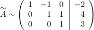
Task. Explore compatibility and find a general solution to the system:

Description of steps:

1. We subtract the first equation from the second (after multiplying by two) and the third - we get the allowed variable x 1;
2. Subtract the second equation from the third. Since all the coefficients in these equations are the same, the third equation will become trivial. At the same time, multiply the second equation by (−1);
3. Subtract the second from the first equation - we get the allowed variable x 2. The entire system of equations is now also resolved;
4. Since the variables x 3 and x 4 are free, we move them to the right to express the allowed variables. This is the answer.

So, the system is consistent and indeterminate, since there are two allowed variables (x 1 and x 2) and two free ones (x 3 and x 4).

Definition and description of the Gaussian method

The Gaussian transformation method (also known as the method of sequential elimination of unknown variables from an equation or matrix) for solving systems of linear equations is a classical method for solving systems of algebraic equations (SLAE). This classical method is also used to solve problems such as obtaining inverse matrices and determining the rank of a matrix.

Transformation using the Gaussian method consists of making small (elementary) sequential changes to a system of linear algebraic equations, leading to the elimination of variables from it from top to bottom with the formation of a new triangular system of equations that is equivalent to the original one.

Definition 1

This part of the solution is called the forward Gaussian solution, since the entire process is carried out from top to bottom.

After reducing the original system of equations to a triangular one, all variables of the system are found from bottom to top (that is, the first variables found are located precisely on the last lines of the system or matrix). This part of the solution is also known as the inverse of the Gaussian solution. His algorithm is as follows: first, the variables closest to the bottom of the system of equations or matrix are calculated, then the resulting values ​​are substituted higher and thus another variable is found, and so on.

Description of the Gaussian method algorithm

The sequence of actions for the general solution of a system of equations using the Gaussian method consists in alternately applying the forward and backward strokes to the matrix based on the SLAE. Let the initial system of equations have the following form:

$\begin(cases) a_(11) \cdot x_1 +...+ a_(1n) \cdot x_n = b_1 \\ ... \\ a_(m1) \cdot x_1 + a_(mn) \cdot x_n = b_m \end(cases)$

To solve SLAEs using the Gaussian method, it is necessary to write the original system of equations in the form of a matrix:

$A = \begin(pmatrix) a_(11) & … & a_(1n) \\ \vdots & … & \vdots \\ a_(m1) & … & a_(mn) \end(pmatrix)$, $b =\begin(pmatrix) b_1 \\ \vdots \\ b_m \end(pmatrix)$

The matrix $A$ is called the main matrix and represents the coefficients of the variables written in order, and $b$ is called the column of its free terms. The matrix $A$, written through a bar with a column of free terms, is called an extended matrix:

$A = \begin(array)(ccc|c) a_(11) & … & a_(1n) & b_1 \\ \vdots & … & \vdots & ...\\ a_(m1) & … & a_( mn) & b_m \end(array)$

Now it is necessary, using elementary transformations on the system of equations (or on the matrix, since this is more convenient), to bring it to the following form:

$\begin(cases) α_(1j_(1)) \cdot x_(j_(1)) + α_(1j_(2)) \cdot x_(j_(2))...+ α_(1j_(r)) \cdot x_(j_(r)) +... α_(1j_(n)) \cdot x_(j_(n)) = β_1 \\ α_(2j_(2)) \cdot x_(j_(2)). ..+ α_(2j_(r)) \cdot x_(j_(r)) +... α_(2j_(n)) \cdot x_(j_(n)) = β_2 \\ ...\\ α_( rj_(r)) \cdot x_(j_(r)) +... α_(rj_(n)) \cdot x_(j_(n)) = β_r \\ 0 = β_(r+1) \\ … \ \ 0 = β_m \end(cases)$ (1)

The matrix obtained from the coefficients of the transformed system of equation (1) is called a step matrix; this is what step matrices usually look like:

$A = \begin(array)(ccc|c) a_(11) & a_(12) & a_(13) & b_1 \\ 0 & a_(22) & a_(23) & b_2\\ 0 & 0 & a_(33) & b_3 \end(array)$

These matrices are characterized by the following set of properties:

1. All its zero lines come after non-zero lines
2. If some row of a matrix with number $k$ is non-zero, then the previous row of the same matrix has fewer zeros than this one with number $k$.

After obtaining the step matrix, it is necessary to substitute the resulting variables into the remaining equations (starting from the end) and obtain the remaining values ​​of the variables.

Basic rules and permitted transformations when using the Gauss method

When simplifying a matrix or system of equations using this method, you need to use only elementary transformations.

Such transformations are considered to be operations that can be applied to a matrix or system of equations without changing its meaning:

• rearrangement of several lines,
• adding or subtracting from one row of a matrix another row from it,
• multiplying or dividing a string by a constant not equal to zero,
• a line consisting of only zeros, obtained in the process of calculating and simplifying the system, must be deleted,
• You also need to remove unnecessary proportional lines, choosing for the system the only one with coefficients that are more suitable and convenient for further calculations.

All elementary transformations are reversible.

Analysis of the three main cases that arise when solving linear equations using the method of simple Gauss transformations

There are three cases that arise when using the Gaussian method to solve systems:

1. When a system is inconsistent, that is, it does not have any solutions
2. The system of equations has a solution, and a unique one, and the number of non-zero rows and columns in the matrix is ​​equal to each other.
3. The system has a certain number or set of possible solutions, and the number of rows in it is less than the number of columns.

Outcome of a solution with an inconsistent system

For this option, when solving a matrix equation using the Gaussian method, it is typical to obtain some line with the impossibility of fulfilling the equality. Therefore, if at least one incorrect equality occurs, the resulting and original systems do not have solutions, regardless of the other equations they contain. An example of an inconsistent matrix:

$\begin(array)(ccc|c) 2 & -1 & 3 & 0 \\ 1 & 0 & 2 & 0\\ 0 & 0 & 0 & 1 \end(array)$

In the last line an impossible equality arose: $0 \cdot x_(31) + 0 \cdot x_(32) + 0 \cdot x_(33) = 1$.

A system of equations that has only one solution

These systems, after being reduced to a step matrix and removing rows with zeros, have the same number of rows and columns in the main matrix. Here is the simplest example of such a system:

$\begin(cases) x_1 - x_2 = -5 \\ 2 \cdot x_1 + x_2 = -7 \end(cases)$

Let's write it in the form of a matrix:

$\begin(array)(cc|c) 1 & -1 & -5 \\ 2 & 1 & -7 \end(array)$

To bring the first cell of the second row to zero, we multiply the top row by $-2$ and subtract it from the bottom row of the matrix, and leave the top row in its original form, as a result we have the following:

$\begin(array)(cc|c) 1 & -1 & -5 \\ 0 & 3 & 10 \end(array)$

This example can be written as a system:

$\begin(cases) x_1 - x_2 = -5 \\ 3 \cdot x_2 = 10 \end(cases)$

The lower equation yields the following value for $x$: $x_2 = 3 \frac(1)(3)$. Substitute this value into the upper equation: $x_1 – 3 \frac(1)(3)$, we get $x_1 = 1 \frac(2)(3)$.

A system with many possible solutions

This system is characterized by a smaller number of significant rows than the number of columns in it (the rows of the main matrix are taken into account).

Variables in such a system are divided into two types: basic and free. When transforming such a system, the main variables contained in it must be left in the left area up to the “=” sign, and the remaining variables must be moved to the right side of the equality.

Such a system has only a certain general solution.

Let us analyze the following system of equations:

$\begin(cases) 2y_1 + 3y_2 + x_4 = 1 \\ 5y_3 - 4y_4 = 1 \end(cases)$

Let's write it in the form of a matrix:

$\begin(array)(cccc|c) 2 & 3 & 0 & 1 & 1 \\ 0 & 0 & 5 & 4 & 1 \\ \end(array)$

Our task is to find a general solution to the system. For this matrix, the basis variables will be $y_1$ and $y_3$ (for $y_1$ - since it comes first, and in the case of $y_3$ - it is located after the zeros).

As basis variables, we choose exactly those that are the first in the row and are not equal to zero.

The remaining variables are called free; we need to express the basic ones through them.

Using the so-called reverse stroke, we analyze the system from bottom to top; to do this, we first express $y_3$ from the bottom line of the system:

$5y_3 – 4y_4 = 1$

$5y_3 = 4y_4 + 1$

$y_3 = \frac(4/5)y_4 + \frac(1)(5)$.

Now we substitute the expressed $y_3$ into the upper equation of the system $2y_1 + 3y_2 + y_4 = 1$: $2y_1 + 3y_2 - (\frac(4)(5)y_4 + \frac(1)(5)) + y_4 = 1$

We express $y_1$ in terms of free variables $y_2$ and $y_4$:

$2y_1 + 3y_2 - \frac(4)(5)y_4 - \frac(1)(5) + y_4 = 1$

$2y_1 = 1 – 3y_2 + \frac(4)(5)y_4 + \frac(1)(5) – y_4$

$2y_1 = -3y_2 - \frac(1)(5)y_4 + \frac(6)(5)$

$y_1 = -1.5x_2 – 0.1y_4 + 0.6$

The solution is ready.

Example 1

Solve slough using the Gaussian method. Examples. An example of solving a system of linear equations given by a 3 by 3 matrix using the Gaussian method

$\begin(cases) 4x_1 + 2x_2 – x_3 = 1 \\ 5x_1 + 3x_2 - 2x^3 = 2\\ 3x_1 + 2x_2 – 3x_3 = 0 \end(cases)$

Let's write our system in the form of an extended matrix:

$\begin(array)(ccc|c) 4 & 2 & -1 & 1 \\ 5 & 3 & -2 & 2 \\ 3 & 2 & -3 & 0\\ \end(array)$

Now, for convenience and practicality, you need to transform the matrix so that $1$ is in the upper corner of the outermost column.

To do this, to the 1st line you need to add the line from the middle, multiplied by $-1$, and write the middle line itself as it is, it turns out:

$\begin(array)(ccc|c) -1 & -1 & 1 & -1 \\ 5 & 3 & -2 & 2 \\ 3 & 2 & -3 & 0\\ \end(array)$

$\begin(array)(ccc|c) -1 & -1 & 1 & -1 \\ 0 & -2 & 3 & -3 \\ 0 & -1 & 0 & -3\\ \end(array) $

Multiply the top and last lines by $-1$, and also swap the last and middle lines:

$\begin(array)(ccc|c) 1 & 1 & -1 & 1 \\ 0 & 1 & 0 & 3 \\ 0 & -2 & 3 & -3\\ \end(array)$

$\begin(array)(ccc|c) 1 & 1 & -1 & 1 \\ 0 & 1 & 0 & 3 \\ 0 & 0 & 3 & 3\\ \end(array)$

And divide the last line by $3$:

$\begin(array)(ccc|c) 1 & 1 & -1 & 1 \\ 0 & 1 & 0 & 3 \\ 0 & 0 & 1 & 1\\ \end(array)$

We obtain the following system of equations, equivalent to the original one:

$\begin(cases) x_1 + x_2 – x_3 = 1\\ x_2 = 3 \\ x_3 = 1 \end(cases)$

From the upper equation we express $x_1$:

$x1 = 1 + x_3 – x_2 = 1 + 1 – 3 = -1$.

Example 2

An example of solving a system defined using a 4 by 4 matrix using the Gaussian method

$\begin(array)(cccc|c) 2 & 5 & 4 & 1 & 20 \\ 1 & 3 & 2 & 1 & 11 \\ 2 & 10 & 9 & 7 & 40\\ 3 & 8 & 9 & 2 & 37 \\ \end(array)$.

At the beginning, we swap the top lines following it to get $1$ in the upper left corner:

$\begin(array)(cccc|c) 1 & 3 & 2 & 1 & 11 \\ 2 & 5 & 4 & 1 & 20 \\ 2 & 10 & 9 & 7 & 40\\ 3 & 8 & 9 & 2 & 37 \\ \end(array)$.

Now multiply the top line by $-2$ and add to the 2nd and 3rd. To the 4th we add the 1st line, multiplied by $-3$:

$\begin(array)(cccc|c) 1 & 3 & 2 & 1 & 11 \\ 0 & -1 & 0 & -1 & -2 \\ 0 & 4 & 5 & 5 & 18\\ 0 & - 1 & 3 & -1 & 4 \\ \end(array)$

Now to line number 3 we add line 2 multiplied by $4$, and to line 4 we add line 2 multiplied by $-1$.

$\begin(array)(cccc|c) 1 & 3 & 2 & 1 & 11 \\ 0 & -1 & 0 & -1 & -2 \\ 0 & 0 & 5 & 1 & 10\\ 0 & 0 & 3 & 0 & 6 \\ \end(array)$

We multiply line 2 by $-1$, and divide line 4 by $3$ and replace line 3.

$\begin(array)(cccc|c) 1 & 3 & 2 & 1 & 11 \\ 0 & 1 & 0 & 1 & 2 \\ 0 & 0 & 1 & 0 & 2\\ 0 & 0 & 5 & 1 & 10 \\ \end(array)$

Now we add to the last line the penultimate one, multiplied by $-5$.

$\begin(array)(cccc|c) 1 & 3 & 2 & 1 & 11 \\ 0 & 1 & 0 & 1 & 2 \\ 0 & 0 & 1 & 0 & 2\\ 0 & 0 & 0 & 1 & 0 \\ \end(array)$

We solve the resulting system of equations:

$\begin(cases) m = 0 \\ g = 2\\ y + m = 2\ \ x + 3y + 2g + m = 11\end(cases)$

In our calculator you will find for free solving a system of linear equations using the Gauss method online with detailed solutions and even complex numbers. With us you can solve both an ordinary definite and an indefinite system of equations, which has an infinite number of solutions. In this case, in the answer you will receive the dependence of some variables through others - free ones. You can also check the system for consistency using the same Gaussian method.

You can read more about how to use our online calculator in the instructions.

About the method

When solving a system of linear equations using the Gaussian method, the following steps are performed.

1. We write the extended matrix.
2. In fact, the algorithm is divided into forward and reverse. A direct move is the reduction of a matrix to a stepwise form. The reverse move is the reduction of the matrix to a special stepwise form. But in practice, it is more convenient to immediately zero out what is located both above and below the element in question. Our calculator uses exactly this approach.
3. It is important to note that when solving using the Gaussian method, the presence in the matrix of at least one zero row with a NON-zero right-hand side (column of free terms) indicates the inconsistency of the system. There is no solution in this case.

To best understand how the algorithm works, enter any example, select "very detailed solution" and study the answer.

The Gaussian method is easy! Why? The famous German mathematician Johann Carl Friedrich Gauss, during his lifetime, received recognition as the greatest mathematician of all time, a genius, and even the nickname “King of Mathematics.” And everything ingenious, as you know, is simple! By the way, not only suckers get money, but also geniuses - Gauss’s portrait was on the 10 Deutschmark banknote (before the introduction of the euro), and Gauss still smiles mysteriously at Germans from ordinary postage stamps.

The Gauss method is simple in that the KNOWLEDGE OF A FIFTH-GRADE STUDENT IS ENOUGH to master it. You must know how to add and multiply! It is no coincidence that teachers often consider the method of sequential exclusion of unknowns in school mathematics electives. It’s a paradox, but students find the Gaussian method the most difficult. Nothing surprising - it’s all about the methodology, and I will try to talk about the algorithm of the method in an accessible form.

First, let's systematize a little knowledge about systems of linear equations. A system of linear equations can:

1) Have a unique solution.
2) Have infinitely many solutions.
3) Have no solutions (be non-joint).

The Gauss method is the most powerful and universal tool for finding a solution any systems of linear equations. As we remember, Cramer's rule and matrix method are unsuitable in cases where the system has infinitely many solutions or is inconsistent. And the method of sequential elimination of unknowns Anyway will lead us to the answer! In this lesson, we will again consider the Gauss method for case No. 1 (the only solution to the system), the article is devoted to the situations of points No. 2-3. I note that the algorithm of the method itself works the same in all three cases.

Let's return to the simplest system from the lesson How to solve a system of linear equations?
and solve it using the Gaussian method.

The first step is to write down extended system matrix:
. I think everyone can see by what principle the coefficients are written. The vertical line inside the matrix does not have any mathematical meaning - it is simply a strikethrough for ease of design.

Reference :I recommend you remember terms linear algebra. System Matrix is a matrix composed only of coefficients for unknowns, in this example the matrix of the system: . Extended System Matrix– this is the same matrix of the system plus a column of free terms, in this case: . For brevity, any of the matrices can be simply called a matrix.

After the extended system matrix is ​​written, it is necessary to perform some actions with it, which are also called elementary transformations.

The following elementary transformations exist:

1) Strings matrices Can rearrange in some places. For example, in the matrix under consideration, you can painlessly rearrange the first and second rows:

2) If there are (or have appeared) proportional (as a special case - identical) rows in the matrix, then you should delete from the matrix all these rows except one. Consider, for example, the matrix . In this matrix, the last three rows are proportional, so it is enough to leave only one of them: .

3) If a zero row appears in the matrix during transformations, then it should also be delete. I won’t draw, of course, the zero line is the line in which all zeros.

4) The matrix row can be multiply (divide) to any number non-zero. Consider, for example, the matrix . Here it is advisable to divide the first line by –3, and multiply the second line by 2: . This action is very useful because it simplifies further transformations of the matrix.

5) This transformation causes the most difficulties, but in fact there is nothing complicated either. To a row of a matrix you can add another string multiplied by a number, different from zero. Let's look at our matrix from a practical example: . First I'll describe the transformation in great detail. Multiply the first line by –2: , And to the second line we add the first line multiplied by –2: . Now the first line can be divided “back” by –2: . As you can see, the line that is ADDED LI – hasn't changed. Always the line TO WHICH IS ADDED changes UT.

In practice, of course, they don’t write it in such detail, but write it briefly:

Once again: to the second line added the first line multiplied by –2. A line is usually multiplied orally or on a draft, with the mental calculation process going something like this:

“I rewrite the matrix and rewrite the first line: »

“First column. At the bottom I need to get zero. Therefore, I multiply the one at the top by –2: , and add the first one to the second line: 2 + (–2) = 0. I write the result in the second line: »

“Now the second column. At the top, I multiply -1 by -2: . I add the first to the second line: 1 + 2 = 3. I write the result in the second line: »

“And the third column. At the top I multiply -5 by -2: . I add the first to the second line: –7 + 10 = 3. I write the result in the second line: »

Please carefully understand this example and understand the sequential calculation algorithm, if you understand this, then the Gaussian method is practically in your pocket. But, of course, we will still work on this transformation.

Elementary transformations do not change the solution of the system of equations

! ATTENTION: considered manipulations can not use, if you are offered a task where the matrices are given “by themselves.” For example, with “classical” operations with matrices Under no circumstances should you rearrange anything inside the matrices!

Let's return to our system. It is practically taken to pieces.

Let us write down the extended matrix of the system and, using elementary transformations, reduce it to stepped view:

(1) The first line was added to the second line, multiplied by –2. And again: why do we multiply the first line by –2? In order to get zero at the bottom, which means getting rid of one variable in the second line.

(2) Divide the second line by 3.

The purpose of elementary transformations – reduce the matrix to stepwise form: . In the design of the task, they just mark out the “stairs” with a simple pencil, and also circle the numbers that are located on the “steps”. The term “stepped view” itself is not entirely theoretical; in scientific and educational literature it is often called trapezoidal view or triangular view.

As a result of elementary transformations, we obtained equivalent original system of equations:

Now the system needs to be “unwinded” in the opposite direction - from bottom to top, this process is called inverse of the Gaussian method.

In the lower equation we already have a ready-made result: .

Let's consider the first equation of the system and substitute the already known value of “y” into it:

Let's consider the most common situation, when the Gaussian method requires solving a system of three linear equations with three unknowns.

Example 1

Solve the system of equations using the Gauss method:

Let's write the extended matrix of the system:

Now I will immediately draw the result that we will come to during the solution:

And I repeat, our goal is to bring the matrix to a stepwise form using elementary transformations. Where to start?

First, look at the top left number:

Should almost always be here unit. Generally speaking, –1 (and sometimes other numbers) will do, but somehow it has traditionally happened that one is usually placed there. How to organize a unit? We look at the first column - we have a finished unit! Transformation one: swap the first and third lines:

Now the first line will remain unchanged until the end of the solution. Now fine.

The unit in the top left corner is organized. Now you need to get zeros in these places:

We get zeros using a “difficult” transformation. First we deal with the second line (2, –1, 3, 13). What needs to be done to get zero in the first position? Need to to the second line add the first line multiplied by –2. Mentally or on a draft, multiply the first line by –2: (–2, –4, 2, –18). And we consistently carry out (again mentally or on a draft) addition, to the second line we add the first line, already multiplied by –2:

We write the result in the second line:

We deal with the third line in the same way (3, 2, –5, –1). To get a zero in the first position, you need to the third line add the first line multiplied by –3. Mentally or on a draft, multiply the first line by –3: (–3, –6, 3, –27). AND to the third line we add the first line multiplied by –3:

We write the result in the third line:

In practice, these actions are usually performed orally and written down in one step:

No need to count everything at once and at the same time. The order of calculations and “writing in” the results consistent and usually it’s like this: first we rewrite the first line, and slowly puff on ourselves - CONSISTENTLY and ATTENTIVELY:


And I have already discussed the mental process of the calculations themselves above.

In this example, this is easy to do; we divide the second line by –5 (since all numbers there are divisible by 5 without a remainder). At the same time, we divide the third line by –2, because the smaller the numbers, the simpler the solution:

At the final stage of elementary transformations, you need to get another zero here:

For this to the third line we add the second line multiplied by –2:


Try to figure out this action yourself - mentally multiply the second line by –2 and perform the addition.

The last action performed is the hairstyle of the result, divide the third line by 3.

As a result of elementary transformations, an equivalent system of linear equations was obtained:

Cool.

Now the reverse of the Gaussian method comes into play. The equations “unwind” from bottom to top.

In the third equation we already have a ready result:

Let's look at the second equation: . The meaning of "zet" is already known, thus:

And finally, the first equation: . “Igrek” and “zet” are known, it’s just a matter of little things:

Answer:

As has already been noted several times, for any system of equations it is possible and necessary to check the solution found, fortunately, this is easy and quick.

Example 2

This is an example for an independent solution, a sample of the final design and an answer at the end of the lesson.

It should be noted that your progress of the decision may not coincide with my decision process, and this is a feature of the Gauss method. But the answers must be the same!

Example 3

Solve a system of linear equations using the Gauss method

Let us write down the extended matrix of the system and, using elementary transformations, bring it to a stepwise form:

We look at the upper left “step”. We should have one there. The problem is that there are no units in the first column at all, so rearranging the rows will not solve anything. In such cases, the unit must be organized using an elementary transformation. This can usually be done in several ways. I did this:
(1) To the first line we add the second line, multiplied by –1. That is, we mentally multiplied the second line by –1 and added the first and second lines, while the second line did not change.

Now at the top left there is “minus one”, which suits us quite well. Anyone who wants to get +1 can perform an additional movement: multiply the first line by –1 (change its sign).

(2) The first line multiplied by 5 was added to the second line. The first line multiplied by 3 was added to the third line.

(3) The first line was multiplied by –1, in principle, this is for beauty. The sign of the third line was also changed and it was moved to second place, so that on the second “step” we had the required unit.

(4) The second line was added to the third line, multiplied by 2.

(5) The third line was divided by 3.

A bad sign that indicates an error in calculations (more rarely, a typo) is a “bad” bottom line. That is, if we got something like , below, and, accordingly, , then with a high degree of probability we can say that an error was made during elementary transformations.

We charge the reverse, in the design of examples they often do not rewrite the system itself, but the equations are “taken directly from the given matrix.” The reverse stroke, I remind you, works from bottom to top. Yes, here is a gift:

Answer: .

Example 4

Solve a system of linear equations using the Gauss method

This is an example for you to solve on your own, it is somewhat more complicated. It's okay if someone gets confused. Full solution and sample design at the end of the lesson. Your solution may be different from my solution.

In the last part we will look at some features of the Gaussian algorithm.
The first feature is that sometimes some variables are missing from the system equations, for example:

How to correctly write the extended system matrix? I already talked about this point in class. Cramer's rule. Matrix method. In the extended matrix of the system, we put zeros in place of missing variables:

By the way, this is a fairly easy example, since the first column already has one zero, and there are fewer elementary transformations to perform.

The second feature is this. In all the examples considered, we placed either –1 or +1 on the “steps”. Could there be other numbers there? In some cases they can. Consider the system: .

Here on the upper left “step” we have a two. But we notice the fact that all the numbers in the first column are divisible by 2 without a remainder - and the other is two and six. And the two at the top left will suit us! In the first step, you need to perform the following transformations: add the first line multiplied by –1 to the second line; to the third line add the first line multiplied by –3. This way we will get the required zeros in the first column.

Or another conventional example: . Here the three on the second “step” also suits us, since 12 (the place where we need to get zero) is divisible by 3 without a remainder. It is necessary to carry out the following transformation: add the second line to the third line, multiplied by –4, as a result of which the zero we need will be obtained.

Gauss's method is universal, but there is one peculiarity. You can confidently learn to solve systems using other methods (Cramer’s method, matrix method) literally the first time - they have a very strict algorithm. But in order to feel confident in the Gaussian method, you need to get good at it and solve at least 5-10 systems. Therefore, at first there may be confusion and errors in calculations, and there is nothing unusual or tragic about this.

Rainy autumn weather outside the window.... Therefore, for everyone who wants a more complex example to solve on their own:

Example 5

Solve a system of four linear equations with four unknowns using the Gauss method.

Such a task is not so rare in practice. I think even a teapot who has thoroughly studied this page will understand the algorithm for solving such a system intuitively. Fundamentally, everything is the same - there are just more actions.

Cases when the system has no solutions (inconsistent) or has infinitely many solutions are discussed in the lesson Incompatible systems and systems with a general solution. There you can fix the considered algorithm of the Gaussian method.

I wish you success!

Solutions and answers:

Example 2: Solution : Let us write down the extended matrix of the system and, using elementary transformations, bring it to a stepwise form.


Elementary transformations performed:
(1) The first line was added to the second line, multiplied by –2. The first line was added to the third line, multiplied by –1. Attention! Here you may be tempted to subtract the first from the third line; I highly recommend not subtracting it - the risk of error greatly increases. Just fold it!
(2) The sign of the second line was changed (multiplied by –1). The second and third lines have been swapped. note, that on the “steps” we are satisfied not only with one, but also with –1, which is even more convenient.
(3) The second line was added to the third line, multiplied by 5.
(4) The sign of the second line was changed (multiplied by –1). The third line was divided by 14.

Reverse:

Answer: .

Example 4: Solution : Let us write down the extended matrix of the system and, using elementary transformations, bring it to a stepwise form:

Conversions performed:
(1) A second line was added to the first line. Thus, the desired unit is organized on the upper left “step”.
(2) The first line multiplied by 7 was added to the second line. The first line multiplied by 6 was added to the third line.

With the second “step” everything gets worse , the “candidates” for it are the numbers 17 and 23, and we need either one or –1. Transformations (3) and (4) will be aimed at obtaining the desired unit

(3) The second line was added to the third line, multiplied by –1.
(4) The third line was added to the second line, multiplied by –3.
(3) The second line was added to the third line, multiplied by 4. The second line was added to the fourth line, multiplied by –1.
(4) The sign of the second line was changed. The fourth line was divided by 3 and placed in place of the third line.
(5) The third line was added to the fourth line, multiplied by –5.

Reverse:

The Gauss method was proposed by the famous German mathematician Carl Friedrich Gauss (1777 - 1855) and is one of the most universal methods for solving SLAEs. The essence of this method is that through successive elimination of unknowns, a given system is transformed into a stepwise (in particular, triangular) system equivalent to the given one. In the practical solution of the problem, the extended matrix of the system is reduced to a stepwise form using elementary transformations over its rows. Next, all the unknowns are found sequentially, starting from bottom to top.

Principle of the Gauss method

The Gauss method includes forward (reducing the extended matrix to a stepwise form, that is, obtaining zeros under the main diagonal) and reverse (obtaining zeros above the main diagonal of the extended matrix) moves. The forward move is called the Gauss method, the reverse move is called the Gauss-Jordan method, which differs from the first only in the sequence of eliminating variables.

The Gauss method is ideal for solving systems containing more than three linear equations, and for solving systems of equations that are not quadratic (which cannot be said about the Cramer method and the matrix method). That is, the Gauss method is the most universal method for finding a solution to any system of linear equations; it works in the case when the system has infinitely many solutions or is inconsistent.

Examples of solving systems of equations

Example

Exercise. Solve SLAE using the Gaussian method.

Solution. Let's write out the extended matrix of the system and, using elementary transformations on its rows, bring this matrix to a stepwise form (forward move) and then perform the reverse move of the Gaussian method (let's make the zeros above the main diagonal). First, let's change the first and second lines so that the element equals 1 (we do this to simplify the calculations):

We divide all elements of the third line by two (or, which is the same thing, multiply by):

From the third line we subtract the second, multiplied by 3:

Multiplying the third line by , we get:

Let us now carry out the reverse of the Gaussian method (Gassou-Jordan method), that is, we will make zeros above the main diagonal. Let's start with the elements of the third column. We need to reset the element to zero; to do this, subtract the third from the second line.